|
|
 |
QP100-01-SR/VIS
100 um Core Diameter, Solarization-Resistant, 200~1100 nm, SMA 905 Connectors, 2 meter
|
|
6-8 Weeks |
$141.00 |
|
|
|
|
QP100-01-XSR/VIS
100 um Core Diameter, Solarization-Resistant, 180~900 nm, SMA 905 Connectors, 2 meter
|
|
6-8 Weeks |
$167.00 |
|
|
|
|
QP200-01-SR/VIS
200 um Core Diameter, Solarization-Resistant, 200~1100 nm, SMA 905 Connectors, 2 meter
|
|
6-8 Weeks |
$141.00 |
|
|
|
|
QP200-01-XSR/VIS
200 um Core Diameter, Solarization-Resistant, 180~900 nm, SMA 905 Connectors, 2 meter
|
|
6-8 Weeks |
$244.00 |
|
|
|
|
QP600-01-SR/VIS2
600 um Core Diameter, Solarization-Resistant, 200~1100 nm, SMA 905 Connectors, 2 meter
|
|
6-8 Weeks |
$192.00 |
|
|
|
|
QP600-01-XSR/VIS
600 um Core Diameter, Solarization-Resistant, 180~900 nm, SMA 905 Connectors, 2 meter
|
|
6-8 Weeks |
$282.00 |
|
|
|
|
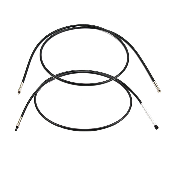
QP-Y-200-2M
Y-Type Fiber Probe, 200 um Core Diameter, 2 meters,200~1100 nm
|
|
6-8 Weeks |
$282.00 |
|
|
|
|
QP-Y-200-2M/XSR
Y-Type Fiber Probe, 200 um Core Diameter, 2 meters, Extreme Solarization-Resistant,180-900nm
|
|
6-8 Weeks |
$385.00 |
|
|
|
|
QP-Y-600-2M
Y-Type Fiber Probe, 600 um Core Diameter, 2 meters, 200~1100 nm
|
|
6-8 Weeks |
$346.00 |
|
|
|
|
QP-Y-600-2M/XSR
Y-Type Fiber Probe, 600 um Core Diameter, 2 meters, Extreme Solarization-Resistant,180-900nm
|
|
6-8 Weeks |
$513.00 |
|
|
|
|
CETO-X
CETO Multi-Function Cuvette Holder, for Abs., Fluo, Raman Use
|
|
6-8 Weeks |
$539.00 |
|
|
|
|
74-UV
UV/VIS Collimating Lens, 200-2000 nm, 5 mm diameter
|
|
6-8 Weeks |
$49.00 |
|
|
|
|
Q-Coli-SM1-SMA
UV/VIS Collimating Lens, SM1 and SMA Connector
|
|
6-8 Weeks |
$257.00 |
|
|
|
|
Q-Coli-SM1-SMA-MVA
UV/VIS Collimating Lens, SM1 and SMA Connector w/ Manual Variable Attenuator
|
|
6-8 Weeks |
$449.00 |
|